Score decomposition

Any strictly proper score decomposes into uncertainty − resolution + reliability (Bröcker, 2009, generalizing the Murphy decomposition of the Brier score to any proper score).

The decomposition

For a forecast $\gamma$ and target $Y$, write:

• $s(p,q) = \sum_k S(p,k)\,q_k$ — expected score of forecast $p$ when $Y \sim q$
• $e(p) = s(p,p)$ — generalized entropy
• $d(p,q) = s(p,q) - e(q)$ — divergence
• $\pi^\gamma = P(Y \mid \gamma)$ — recalibrated forecast
• $\bar\pi = \mathbb{E}[\pi^\gamma]$ — climatology (the marginal of $Y$)

Then Bröcker’s Eq. (13), for any strictly proper loss $S$, is

It is the Savage split $s(\gamma, \pi^\gamma) = e(\pi^\gamma) + d(\gamma, \pi^\gamma)$, then $\mathbb{E}[e(\pi^\gamma)] = e(\bar\pi) - \mathbb{E}[d(\bar\pi, \pi^\gamma)]$ by linearity of $s(\bar\pi, \cdot)$.

Cross-entropy

The log score sets $s(p,q) = H(q,p)$, $e(p) = H(p)$, $d(p,q) = \mathrm{KL}(q \,\|\, p)$, giving

• Uncertainty — the base-rate entropy $H(Y)$
• Resolution — the mutual information $I(Y;\gamma)$ between output and target
• Reliability — the calibration gap $\mathbb{E}[\mathrm{KL}(\pi^\gamma \,\|\, \gamma)]$, zero iff $\gamma = \pi^\gamma$

A constant forecast scores $H(Y)$; an oracle maximizes $I(Y;\gamma)$ and zeroes the gap.

How it’s estimated

Resolution and reliability both need $\pi^\gamma$, which we don’t have in closed form. We estimate it by bucketing: $\gamma$ is the model’s predicted distribution, $Y$‘s marginal is the dataset disease base rate, and $\pi^\gamma$ is each $\gamma$-bucket’s empirical gold rate. The decomposition is therefore an estimate (bucket-dependent), but the ordering of methods holds across choices.

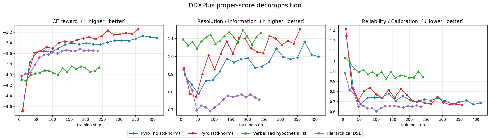
On DDXPlus